All of these algorithms are "greedy," meaning that at each step, the algorithm chooses whichever option is most appealing at that point. Nearest-neighbor, Prim, and Dijkstra "grow" the circuit or tree out from a starting vertex. In other words, they have a "local" focus; at each step, we only consider those edges adjacent to previously chosen vertices, choosing the cheapest option which satisfies our needs. Meanwhile, sorted-edges and Kruskal are "global" algorithms, meaning that each edge is (greedily) chosen from the entire graph. (Actually, Dijkstra might be viewed as having some global aspect, as noted below.)
For the Traveling Salesman Problem (TSP), we imagine that each vertex is a city, the edges represent roads, and the weights of the edges are the distances (or cost of traveling on that road). The goal is to find the minimum-cost Hamiltonian circuit; that is, a sequence of edges which allows the salesman to visit each city exactly once before returning to the city of origin—hopefully traveling the smallest possible distance in the process. The nearest-neighbor and sorted-edges algorithms typically find a low-cost circuit, although they might not find the minimum cost circuit; only a brute-force search—trying every possible route—can guarantee that. (This is because the greedy choices made by these algorithms sometimes force more expensive choices later in the process.) This page only applies these algorithms on complete graphs; that is, graphs in which every pair of vertices are connected by a unique edge.
For any graph, a spanning tree is collection of edges sufficient to provide exactly one path between every pair of vertices. This restriction means that there can be no circuits formed by the chosen edges.
 A minimum-cost spanning tree is one which has the smallest possible total weight (where weight represents cost or distance). There might be more than one such tree, but Prim and Kruskal are both guaranteed to find one of them.
For a specified vertex (say X), a shortest path tree is a spanning tree such that the path from X to any other vertex is as short as possible (i.e., has the minimum possible weight).
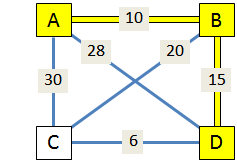
Minimum-cost trees and shortest-path trees are easily confused, as are the Prim and Dijkstra algorithms that solve them. Both algorithms "grow out" from the starting vertex, at each step choosing an edge which connects a vertex Y which is in the tree to a vertex Z which is not. However, while Prim chooses the cheapest such edge, Dijkstra chooses the edge which results in the shortest path from X to Z. A simple illustration is helpful to understand the difference between these algorithms and the trees they produce. In the graph on the right, starting from the vertex A, both Prim and Dijkstra begin by choosing edge AB, and then adding edge BD. Here is where the two algorithms diverge: Prim completes the tree by adding edge DC, while Dijkstra adds either AC or BC, because paths A-C and A-B-C (both with total distance 30) are shorter than path A-B-D-C (total distance 31).
| Algorithm approach | ||
|---|---|---|
| Global | Local | |
| TSP |
Sorted edges: At each step, choose the cheapest available edge anywhere which does not violate the goal of creating a Hamiltonian circuit. |
Nearest neighbor: At each step, choose the cheapest available edge attached to the most recent vertex which does not violate the goal of creating a Hamiltonian circuit. |
| Minimum cost spanning tree |
Kruskal: At each step, choose the cheapest available edge anywhere which does not violate the goal of creating a spanning tree. |
Prim: At each step, choose the cheapest available edge attached to any previously chosen vertex which does not violate the goal of creating a spanning tree. |
| Shortest path spanning tree |
Dijkstra: At each step, choose the edge attached to any previously chosen vertex (the local aspect) which makes the total distance from the starting vertex (the global aspect) as small as possible, and does not violate the goal of creating a spanning tree. |
|