Instructions

This page allows you to do Monte Carlo simulations of a queueing process, by specifying:

• The arrival-time distribution*
• The service-time distribution*
• The number of servers
• The initial length of the queue
• The maximum length of the queue

*Note that if an exponential distribution is chosen, the rate can be given as a function of n, the current length of the queue. For example, the entry λ_n = 1/(n+1) would mean that arrivals slow down as the line gets longer. An entry of the form [1,0.6,0.4,0.2] would result in λ₀ = 1, λ₁ = 0.6, λ₂ = 0.4, and λ_n = 0.2 for n≥3.

Given this information, we simulate 10000 iterations of this queue (out until the specified maximum time), and keep track of the queue length at various points over that interval.

The results of the simulation are displayed graphically in two ways:

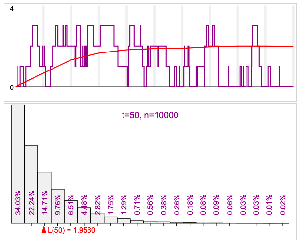
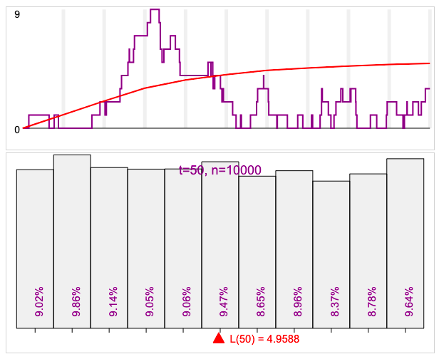
• an example of one simulated queue (showing how the length of the queue increases and decreases over time), with the mean length superimposed over in red.
• a histogram showing the distribution of line length at various points in time.

In some cases, the queue length distribution approaches a stable distribution as t→∞. Specifically, this can happen:

• when the servers are able to keep up with the arrivals. In the first graph below, the service rate is 50% higher than the arrival rate.
• when the length of the queue has an upper limit. In the second graph, the arrival and service rates are equal, but the queue length is capped at 10, so in the limit, the length is uniformly distributed from 0 to 10 (11 possible values).

Note: The first link for each of these examples opens in a separate tab. The second link will overwrite the current model in this tab—so don't use it if you have created a model that you want to save!

1. Service occurs at a constant rate, arrival rate is inversely proportional to (1+n).
   This simulates a line with a single server, where people are increasingly reluctant to join the line the longer it gets. The theoretical steady-state distribution is 1/e, 1/e, 1/2e, 1/6e, ...—that is, P(S=k) = 1/(e k!).
   open in new tab | overwrite current model
2. Constant service rate, arrival rate inversely proportional to sqrt(n+1).
   In this model, people are again reluctant to join when the line as long, but the effect is not as large. The approximate stable distribution is 0.2882, 0.2882, 0.2038, 0.1177, 0.0588, 0.0263, ... (after the first two probabilities, divide by √2, then √3, etc.).
   open in new tab | overwrite current model

Release history

This page was created for demonstration and exploration purposes when I first taught Bluffton's Operations Research course (MAT360) in the fall semester of 2018. A few minor updates were made in Fall 2024 (as I am teaching that class again).

October 2, 2024: Corrected a flaw in the algorithm for generating gamma random variables. Added buttons to copy the plots to the clipboard.

Troubleshooting and technical details

I'll add more technical details here—once I've refreshed my memory as to how I wrote this code 6 years ago!